library(readxl)
BVBRC <- read_xlsx("BVBRC_sp_gene.xlsx")
DGEmBio <- read_xlsx("mbio.01699-24-s0002.xlsx")Data wrangling
Created Nov 2024, Last updated: 18 November, 2025
What is this page for?
This page has code for session 2 of BPI stats workshop. These exercises will only work if you have completed the pre-session items described here correctly. Go to the Session 1 instructions before these exercises.
Data
We will use our published E. cloacae RNAseq data, which can be downloaded from the journal mBio (Choi & Bennison et al, 2024, mBio 0:e01699-24) to perform data wrangling with base R and tidyverse. Get the differential gene expression (DGE) data from supplementary info. Or download the file locally from here. Import this file with read_excel and save as DGEmBio.
Get genome annotation data for speciality genes in E. cloacae ATCC 13047 from BVBRC (Bacterial & Viral Bioinformatics Resource Centre) or locally from here. Import this file with read_excel and save as BVBRC.
We will also use the data table that we used in Session 1, which is in wide format.
Table summaries with group_by and aggregate
We use the data_2w_festing table as an example to obtain mean and SD (or any other summary) for grouped data.
library(grafify) #for datasetLoading required package: ggplot2library(dplyr) #for group_by() and summarise() calls
Attaching package: 'dplyr'The following objects are masked from 'package:stats':
filter, lagThe following objects are masked from 'package:base':
intersect, setdiff, setequal, union#tidyverse way with group_by and chaining
data_2w_Festing |> #this is the base R `pipe`
group_by(Strain, Treatment) |> #grouping by levels
summarise(M = mean(GST), #desired calculations
SD = sd(GST))`summarise()` has grouped output by 'Strain'. You can override using the
`.groups` argument.# A tibble: 8 × 4
# Groups: Strain [4]
Strain Treatment M SD
<fct> <fct> <dbl> <dbl>
1 129/Ola Control 526. 112.
2 129/Ola Treated 742. 33.2
3 A/J Control 508. 142.
4 A/J Treated 929 103.
5 BALB/C Control 504. 115.
6 BALB/C Treated 704. 111.
7 NIH Control 604 226.
8 NIH Treated 722. 153. #table_summary() is an easy function in grafify
table_summary(data = data_2w_Festing,
Ycol = "GST",
ByGroup = c("Strain", "Treatment")) Strain Treatment GST.Mean GST.Median GST.SD GST.Count
1 129/Ola Control 526.5 526.5 112.42998 2
2 A/J Control 508.5 508.5 142.12846 2
3 BALB/C Control 504.5 504.5 115.25841 2
4 NIH Control 604.0 604.0 226.27417 2
5 129/Ola Treated 742.5 742.5 33.23402 2
6 A/J Treated 929.0 929.0 103.23759 2
7 BALB/C Treated 703.5 703.5 111.01576 2
8 NIH Treated 722.5 722.5 153.44217 2#base R method aggregate()
aggregate(data_2w_Festing["GST"], #Y variable
by = data_2w_Festing[c("Strain", "Treatment")], #grouping variables
FUN = function(x){c(M = mean(x), #summaries
SD = sd(x))}) Strain Treatment GST.M GST.SD
1 129/Ola Control 526.50000 112.42998
2 A/J Control 508.50000 142.12846
3 BALB/C Control 504.50000 115.25841
4 NIH Control 604.00000 226.27417
5 129/Ola Treated 742.50000 33.23402
6 A/J Treated 929.00000 103.23759
7 BALB/C Treated 703.50000 111.01576
8 NIH Treated 722.50000 153.44217Converting Long tables to Wide
In R, data for graphing and statistical analyses have to be in long format. The long and wide formats are inter-convertible with tidyr package. There is a base R function (reshape), but in this case I prefer the tidyr versions, which have a more intuitive syntax.
Long table to wide
#tidyverse way
library(tidyr)          #for pivot_wider() and pivot_longer()
#widen data_2w_festing
pivot_wider(data = data_2w_Festing,
            names_from = Treatment,
            values_from = GST)
# A tibble: 8 × 4
Block Strain Control Treated
<fct> <fct> <int> <int>
1 A NIH 444 614
2 A BALB/C 423 625
3 A A/J 408 856
4 A 129/Ola 447 719
5 B NIH 764 831
6 B BALB/C 586 782
7 B A/J 609 1002
8 B 129/Ola 606 766#base R method, not recommended
#the tidyverse method is easier to remember
reshape(data = data_2w_Festing,
idvar = c("Strain", "Block"),
timevar = "Treatment",
direction = "wide") Block Strain GST.Control GST.Treated
1 A NIH 444 614
3 A BALB/C 423 625
5 A A/J 408 856
7 A 129/Ola 447 719
9 B NIH 764 831
11 B BALB/C 586 782
13 B A/J 609 1002
15 B 129/Ola 606 766Wide table to long
In this case, we will use the Weights data table from Session 1.
#tidyverse way
Weights %>%           # this is the tidyverse `pipe`
  pivot_longer(cols = c("chow", "fat"),
               names_to = "Diet",
               values_to = "Bodyweight")
# A tibble: 20 × 3
Mouse Diet Bodyweight
<chr> <chr> <dbl>
1 A chow 29.9
2 A fat 28.3
3 B chow 27.3
4 B fat 29.0
5 C chow 24.0
6 C fat 29.0
7 D chow 24.8
8 D fat 24.6
9 E chow 25.2
10 E fat 34.6
11 F chow 20.4
12 F fat 28.1
13 G chow 22.7
14 G fat 28.8
15 H chow 23.5
16 H fat 31.1
17 I chow 26.1
18 I fat 27.7
19 J chow 32.0
20 J fat 35.0Ordering (sorting) rows
For this exercise and steps below, we will use the DGE tables we downloaded earlier. Ensure you have imported the tables and saved them as DGEmBio and BVBRC as above.
Here is how we can reorder rows in ascending or descending order alphabetically or numerically.
#by increasing logFC
DGEmBio <- DGEmBio[order(-DGEmBio$logFC),]
Merging tables
The BVBRC table has additional description of gene function in “specialty categories”. This is stored in the column “Property”. We want to bring this information for the genes that are differentially expressed in our RNAseq. This is called merging or joining tables.
We want to bring in the column Property from the table BVBRC into the table DGEmBio by matching the gene names. This info is in the columns RefSeq Locus Tag and gene_id in the tables BVBRC and DGEmBio, respectively.
# join with gene name
mBioMerge <- merge(x = DGEmBio,
                  y = BVBRC[c(2,6)],
                  by.x = "gene_id",
                  by.y = "RefSeq Locus Tag",
                  all.x = TRUE)
library(dplyr)
mBioJoin <- left_join(x = DGEmBio,
                      y = BVBRC[c(2,6)],
                      by = c("gene_id" = "RefSeq Locus Tag"))
Create new columns based on conditions
To be able to map additional information on DGEs in a volcano plot, we would like create a variable called Expression, which has high, low or medium when logFC gene expression is >= 4, <= -4 or between this range, respectively.
#create Expression with "high" and "low"
mBioMerge$Expression[mBioMerge$logFC >= 4] <- "high"
mBioMerge$Expression[mBioMerge$logFC <= -4] <- "low"
mBioMerge$Expression[mBioMerge$logFC > -4 &
                        mBioMerge$logFC < 4] <- "medium"

#alternative is transform()
mBioJoin <- transform(mBioJoin,
                      Expression = ifelse(mBioJoin$logFC >= 4, "high",
                                          ifelse(mBioJoin$logFC <= -4, "low",
                                                 ifelse((mBioJoin$logFC < 4 &
                                                          mBioJoin$logFC > -4), "medium", ""))))
Plots
Volcano plot
Here’s a way to make a volcano plot using the processed data frame (mBioMerge) from above. This is quite conveniently done with plot_xy_catgroup from grafify.
#volcano plot
plot_xy_CatGroup(mBioMerge,
                 logFC,
                 -log10(adj.P.Val),
                 Expression,
                 fontsize = 16)+
  labs(title = "Volcano plot")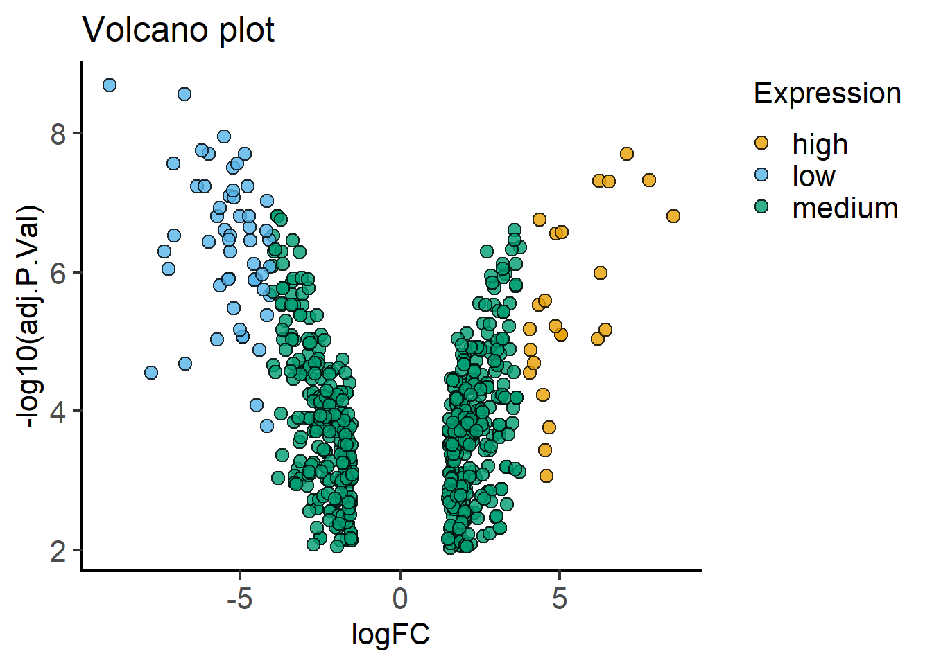
plot_xy_CatGroup(mBioMerge,
                 logFC,
                 -log10(adj.P.Val),
                 Property,
                 ColPal = "vibrant",
                 fontsize = 16)+
  labs(title = "Volcano plot")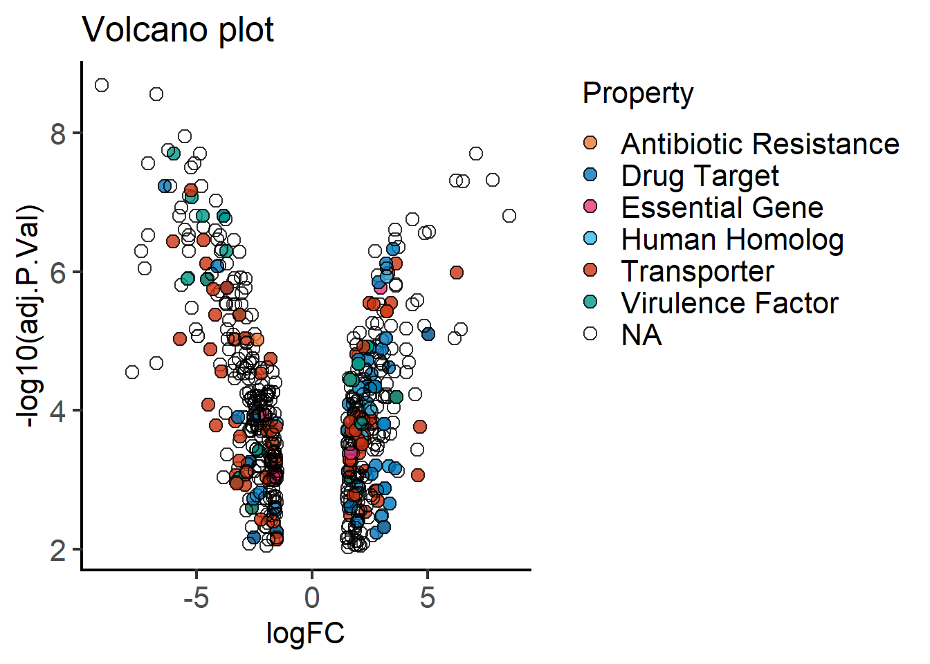
plot_xy_NumGroup(mBioMerge,
                 start,
                 logFC,
                 logFC,
                 ColPal = "Pr")+
  coord_polar()+                     #makes a circular X axis
  labs(title = "Genome-wide DGEs",
       x = "Gene start position")+
  theme_minimal(base_size = 14)
Warning: `coord_polar()` cannot render guide for the aesthetic: x.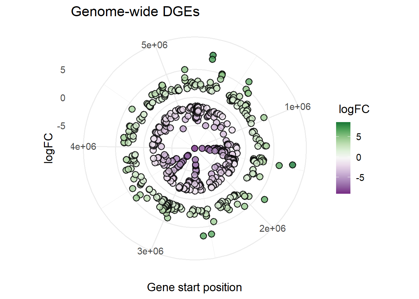
Plotting with ggplot2
One of the advantages of ggplot2 is the ability to easily add additional variables to a graph by mapping them to colour, shape, size of symbols etc.
We are going to do more data wrangling to create an additional variable DNAend for plotting the DGE data across the whole genome of E. cloacae. The values are the contig lengths for ATCC 13047 strain as annotated by BVBRC.
mBioMerge$DNAEnd[mBioMerge$seqid == "Chromosome"] <- 5314581
mBioMerge$DNAEnd[mBioMerge$seqid == "pECL_A"] <- 199562
mBioMerge$DNAEnd[mBioMerge$seqid == "pECL_B"] <- 84653
#adding multiple variables
ggplot(mBioMerge,
       aes(x = start,
           y = logFC))+
  geom_rect(aes(xmin = 0, xmax = DNAEnd,
                ymin = -0.5, ymax = 0.5),
            fill = "grey95")+
  geom_point(aes(fill = logFC),
             size = 2,
             shape = 22)+
  scale_fill_grafify(palette = "PrGn_div")+
  coord_polar()+
  labs(title = "Genome-wide DGEs",
       x = "Gene start position")+
  facet_wrap(~seqid,
             scales = "free_x")+
  theme_minimal(base_size = 10)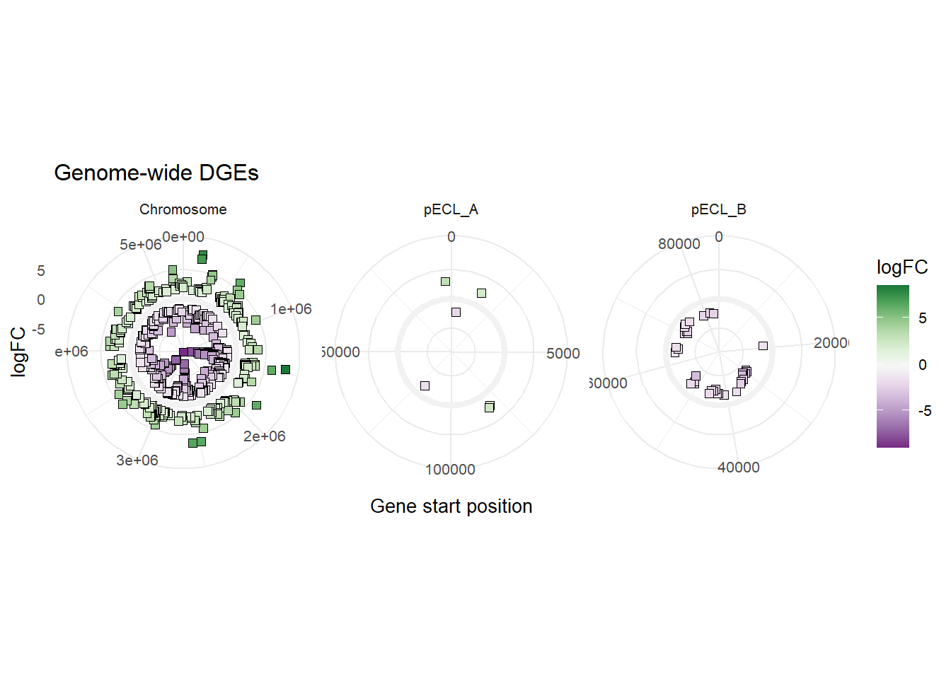
#colour by Property
ggplot(mBioMerge,
       aes(x = start,
           y = logFC))+
  geom_point(aes(fill = Property),
             shape = 21,
             size = 4)+
  scale_fill_grafify(palette = "bright")+
  coord_polar()+
  labs(title = "Genome-wide DGEs",
       x = "Gene start position")+
  theme_minimal(base_size = 14)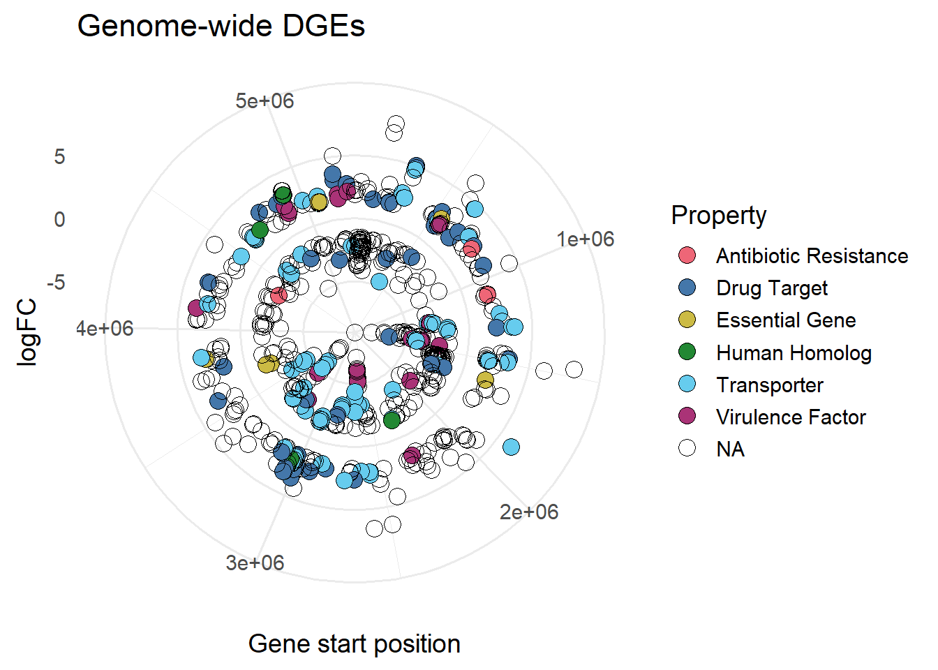
#size based on LogFC
ggplot(mBioMerge,
       aes(x = start,
           y = logFC))+
  geom_point(aes(fill = Property,
                 size = logFC),
             shape = 21)+
  scale_fill_grafify(palette = "bright")+
  coord_polar()+
  labs(title = "Genome-wide DGEs",
       x = "Gene start position")+
  theme_minimal(base_size = 14)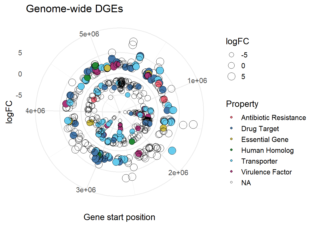
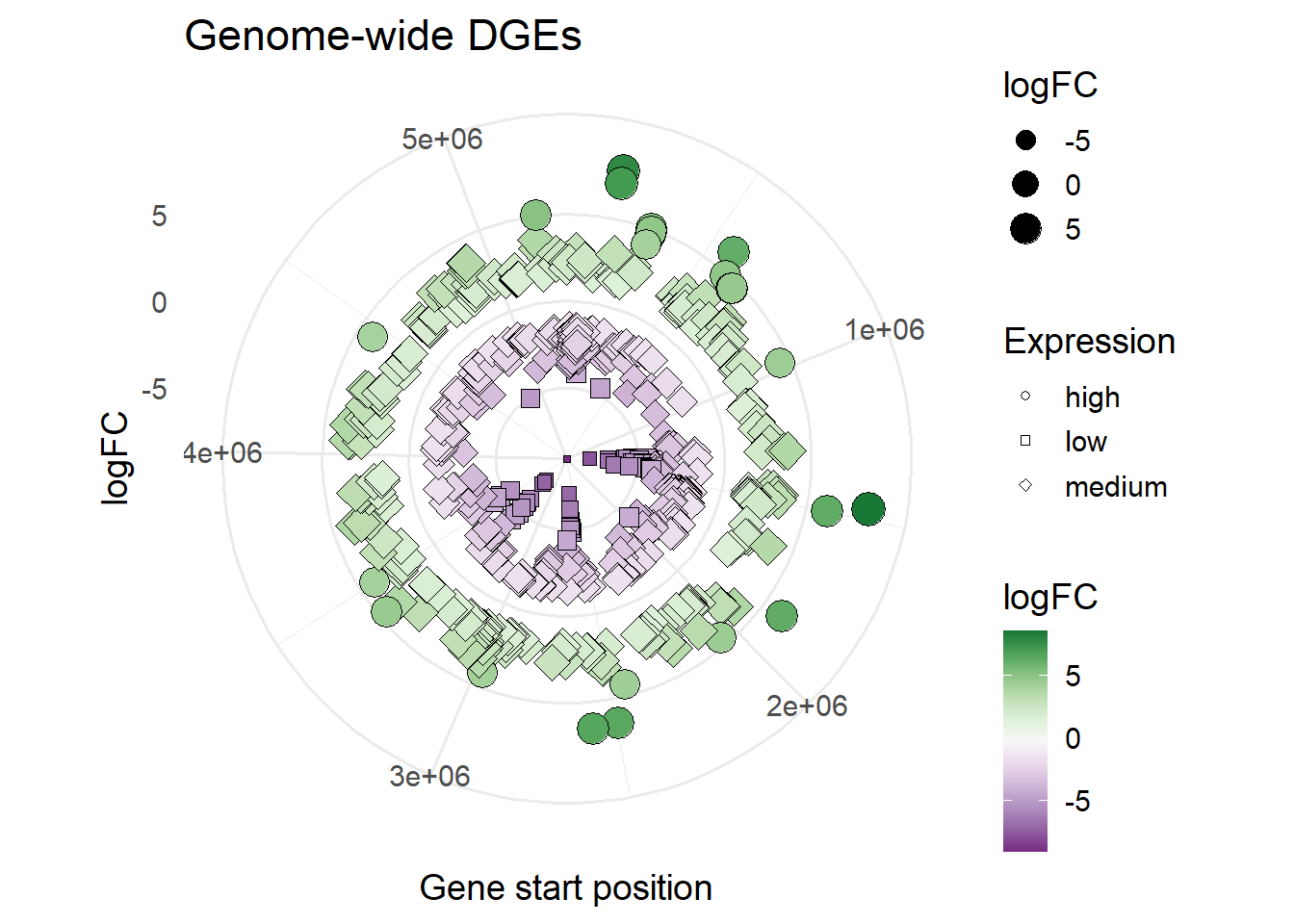
#shape based on Expression
ggplot(mBioMerge,
       aes(x = start,
           y = logFC))+
  geom_point(aes(size = logFC,
                 fill = logFC,
                 shape = Expression))+
  scale_fill_grafify(palette = "PrGn_div")+
  scale_shape_manual(values = 21:23)+
  coord_polar()+
  labs(title = "Genome-wide DGEs",
       x = "Gene start position")+
  theme_minimal(base_size = 14)