We use cookies to measure anonymised site visitor numbers and usage, which help us improve user experience.

Accept cookies?

Linear Models

Linear models

t test

A Student’s t test.

library(grafify)

Loading required package: ggplot2

t.test(Bodyweight ~ Diet, 
       Weights_long)

    Welch Two Sample t-test

data:  Bodyweight by Diet
t = -2.7058, df = 17.892, p-value = 0.01453
alternative hypothesis: true difference in means between group chow and group fat is not equal to 0
95 percent confidence interval:
 -7.1178367 -0.8941633
sample estimates:
mean in group chow  mean in group fat 
            25.603             29.609 

Linear model

#grafify linear model
simple_model(Weights_long,
             "Bodyweight",
             "Diet")

Call:
lm(formula = Bodyweight ~ Diet, data = Weights_long)

Coefficients:
(Intercept)      Dietfat  
     25.603        4.006  

#grafify anova table
simple_anova(Weights_long,
             "Bodyweight",
             "Diet")

Anova Table (Type II tests)

Response: Bodyweight
          Sum Sq Mean sq Df F value  Pr(>F)  
Diet       80.24   80.24  1  7.3212 0.01447 *
Residuals 197.28   10.96 18                  
---
Signif. codes:  0 '***' 0.001 '**' 0.01 '*' 0.05 '.' 0.1 ' ' 1

#lm with formula
lm(Bodyweight ~ Diet, 
   data = Weights_long)

Call:
lm(formula = Bodyweight ~ Diet, data = Weights_long)

Coefficients:
(Intercept)      Dietfat  
     25.603        4.006  

#anova table
anova(lm(Bodyweight ~ Diet, 
         data = Weights_long))

Analysis of Variance Table

Response: Bodyweight
          Df Sum Sq Mean Sq F value  Pr(>F)  
Diet       1  80.24   80.24  7.3212 0.01447 *
Residuals 18 197.28   10.96                  
---
Signif. codes:  0 '***' 0.001 '**' 0.01 '*' 0.05 '.' 0.1 ' ' 1

You can get more information on the linear model with the summary command. To be able to run this, and other diagnostics, you must first save the model as an object in your environment.

#save the model
#grafify linear model
lmod1 <- simple_model(Weights_long,
                      "Bodyweight",
                      "Diet")
#get detailed summary
summary(lmod1)

Call:
lm(formula = Bodyweight ~ Diet, data = Weights_long)

Residuals:
   Min     1Q Median     3Q    Max 
-5.243 -1.667 -0.694  1.538  6.417 

Coefficients:
            Estimate Std. Error t value Pr(>|t|)    
(Intercept)   25.603      1.047  24.456 2.92e-15 ***
Dietfat        4.006      1.481   2.706   0.0145 *  
---
Signif. codes:  0 '***' 0.001 '**' 0.01 '*' 0.05 '.' 0.1 ' ' 1

Residual standard error: 3.311 on 18 degrees of freedom
Multiple R-squared:  0.2891,    Adjusted R-squared:  0.2496 
F-statistic: 7.321 on 1 and 18 DF,  p-value: 0.01447

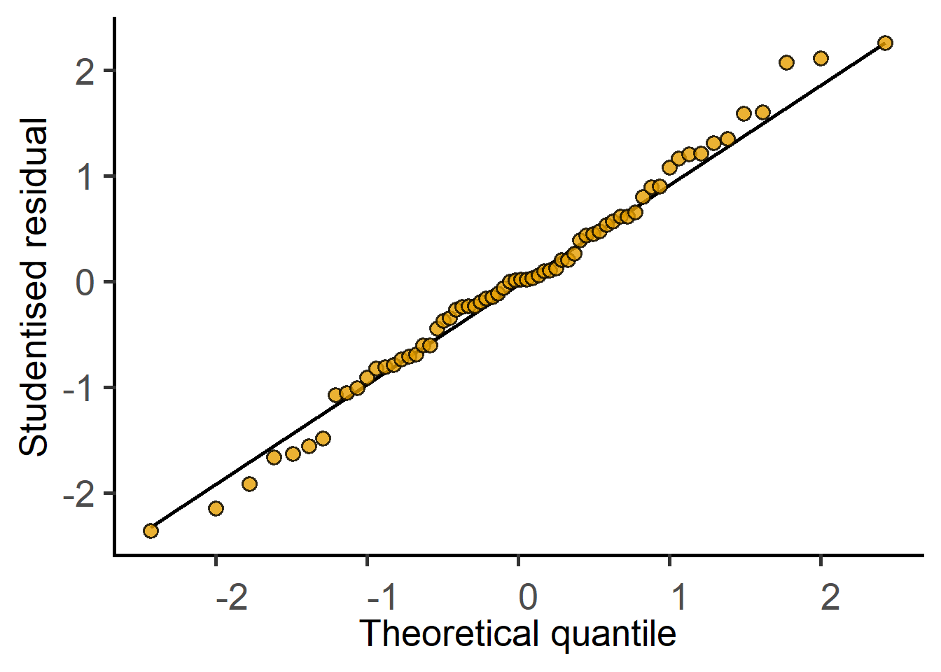
#get a residuals plot
plot_qqmodel(lmod1)

Diagnosing a linear model with a plot of residuals

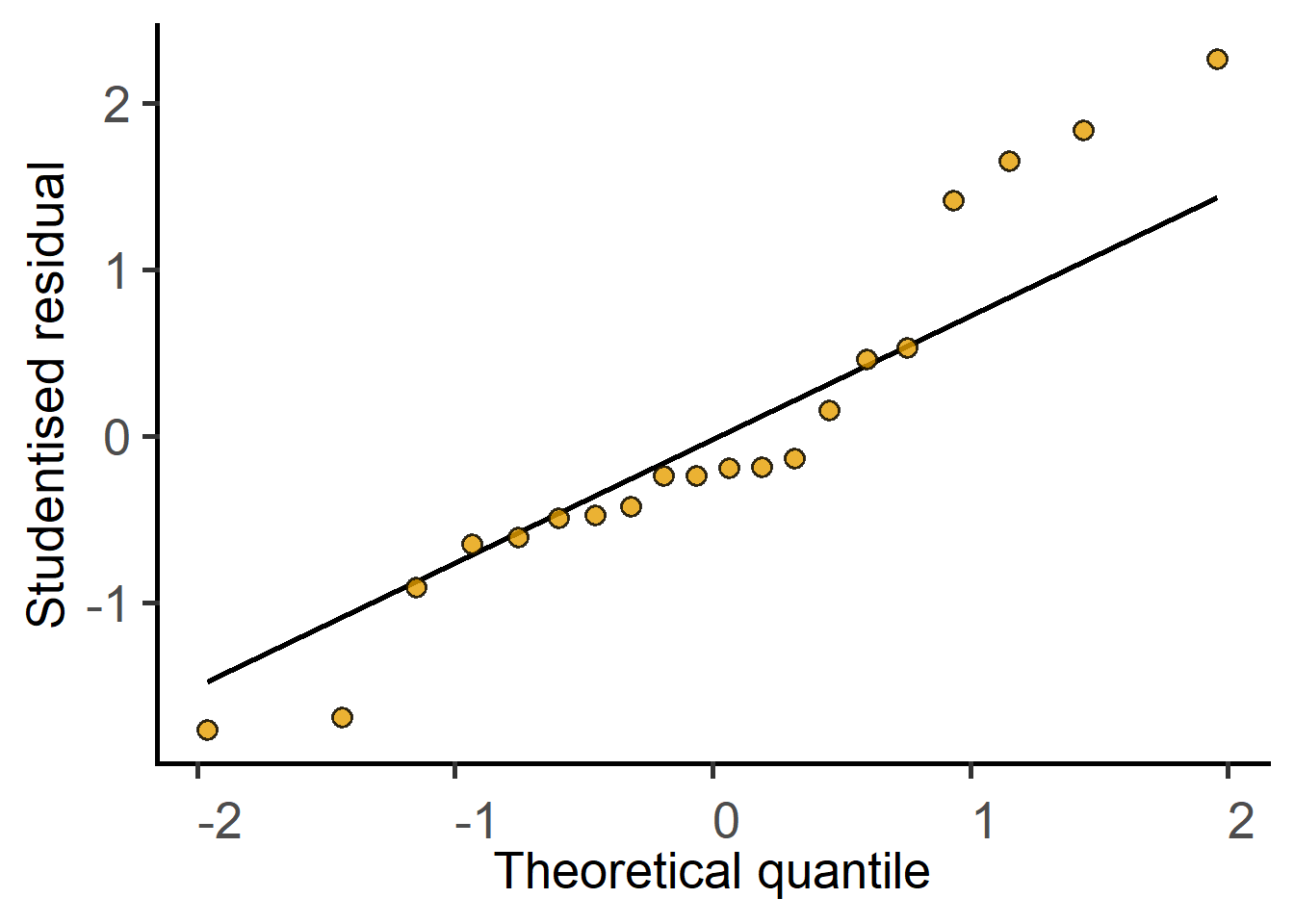
The residuals of the model fit should be assessed after the test. For a test result to be reliable, the residuals should be normally (or approximately normally) distributed.

Here we will use the data_t_pratio table.

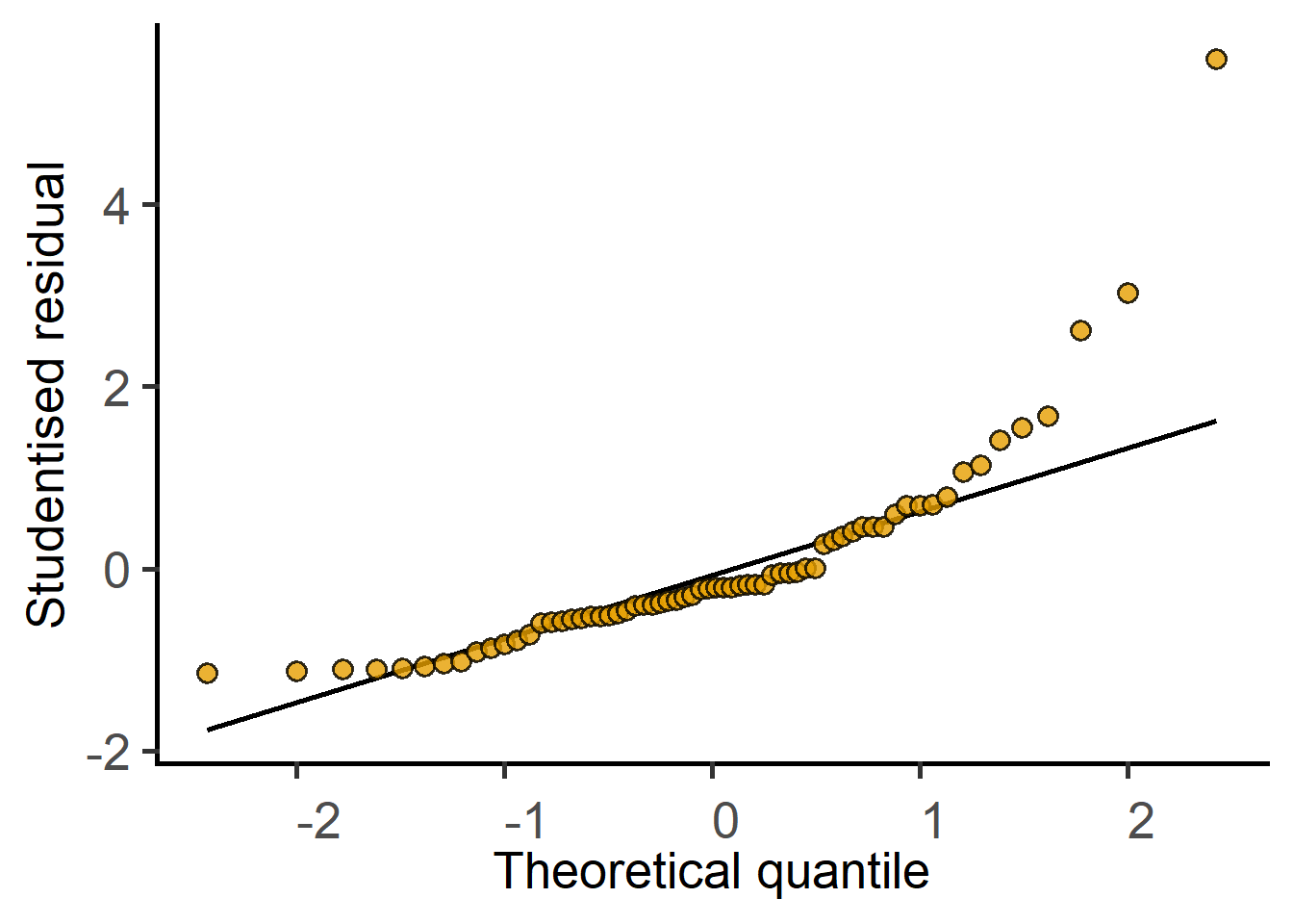
#fit model 1
lin.m1 <- simple_model(data = data_t_pratio,
                       Y_value = "Cytokine",
                       Fixed_Factor = "Genotype")
#fit a model of log-transformed data
lin.m2 <- simple_model(data = data_t_pratio,
                       Y_value = "log(Cytokine)",
                       Fixed_Factor = "Genotype")
#plot residuals of both models
plot_qqmodel(lin.m1) #original data

plot_qqmodel(lin.m2) #log-transformed data

Mixed effects models

Here, our data are matched by Experiment. We can use mixed effects models with Experiment as a random factor.

#fit mixed model 1
mx.lin.m1 <- mixed_model(data = data_t_pratio,
                         Y_value = "Cytokine",
                         Fixed_Factor = "Genotype",
                         Random_Factor = "Experiment")

The new argument `AvgRF` is set to TRUE by default in >=5.0.0). Response variable is averaged over levels of Fixed and Random factors. Use help for details.

#fit a model of log-transformed data
mx.lin.m2 <- mixed_model(data = data_t_pratio,
                         Y_value = "log(Cytokine)",
                         Fixed_Factor = "Genotype",
                         Random_Factor = "Experiment")

The new argument `AvgRF` is set to TRUE by default in >=5.0.0). Response variable is averaged over levels of Fixed and Random factors. Use help for details.

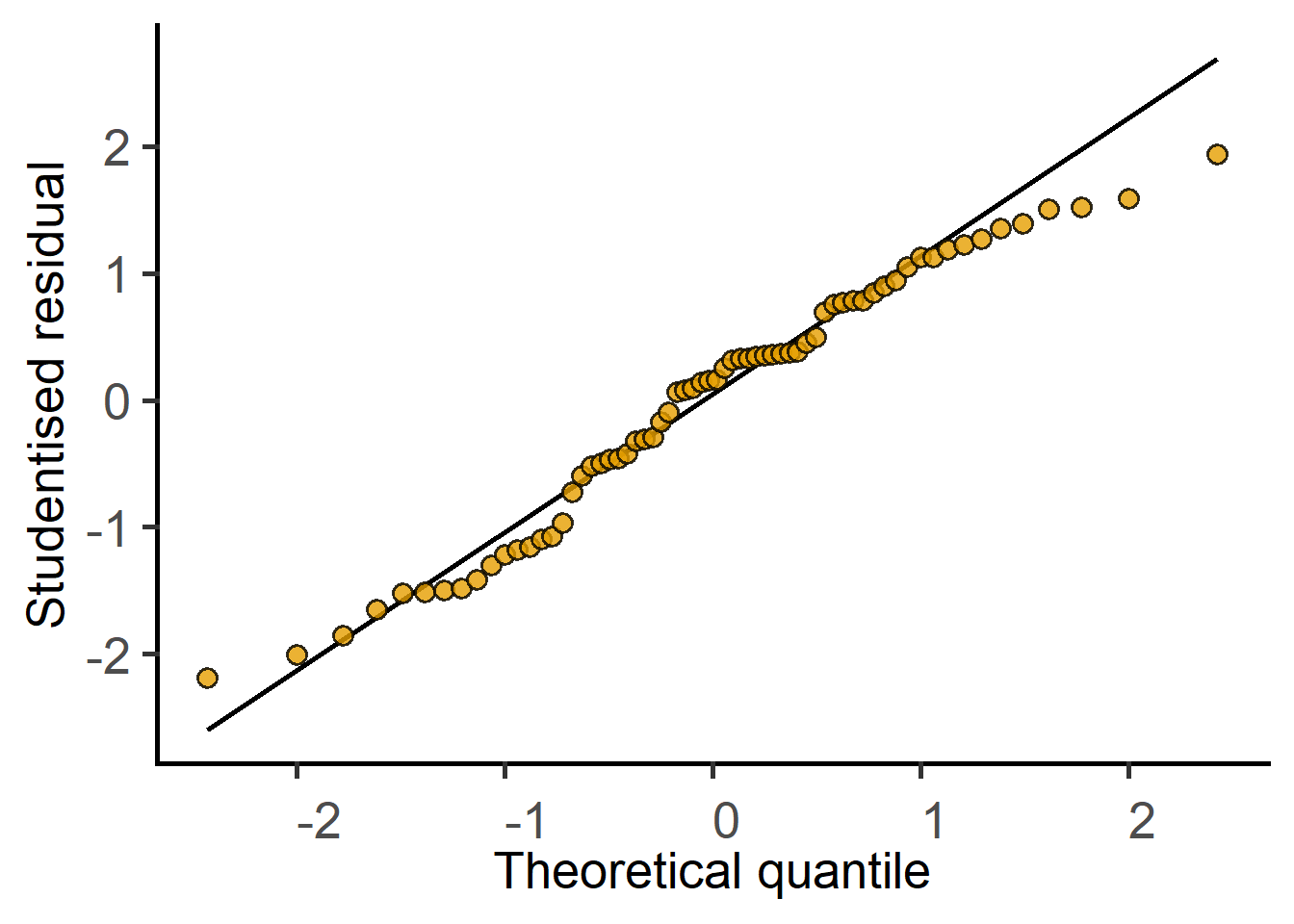
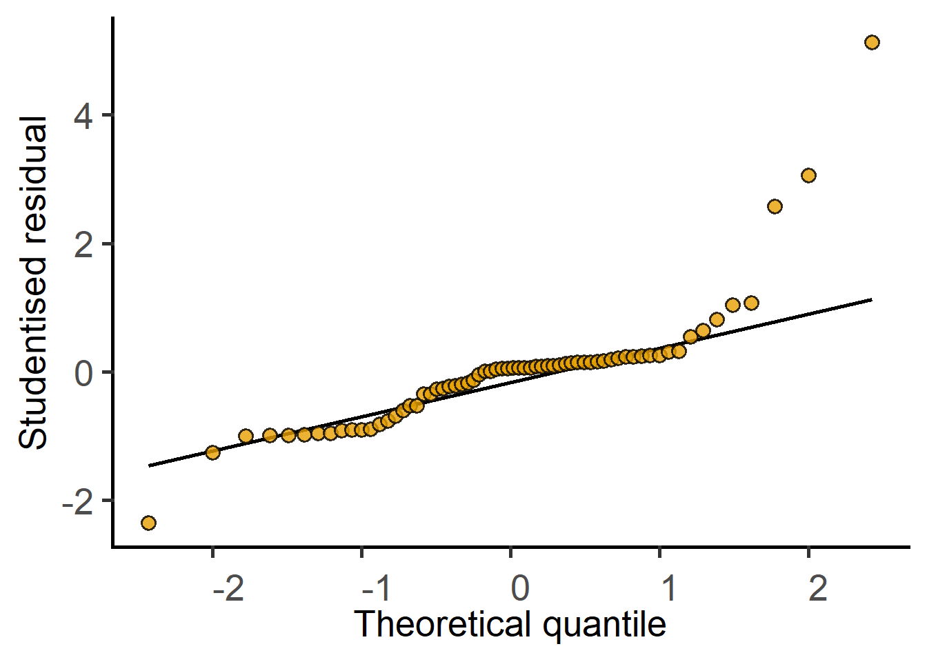
#plot residuals of both models
plot_qqmodel(mx.lin.m1) #original data

plot_qqmodel(mx.lin.m2) #log-transformed data

ANOVA tables

In grafify, you can use very similar code to get ANOVA tables as for fitting a model. Once you diagnose which model fits the data better, use that one to get the ANOVA table and post-hoc comparisons.

mixed_anova(data = data_t_pratio,
            Y_value = "log(Cytokine)",
            Fixed_Factor = "Genotype",
            Random_Factor = "Experiment")

The new argument `AvgRF` is set to TRUE by default in >=5.0.0). Response variable is averaged over levels of Fixed and Random factors. Use help for details.

Type II Analysis of Variance Table with Kenward-Roger's method
         Sum Sq Mean Sq NumDF DenDF F value    Pr(>F)    
Genotype 6.4867  6.4867     1    32  68.873 1.758e-09 ***
---
Signif. codes:  0 '***' 0.001 '**' 0.01 '*' 0.05 '.' 0.1 ' ' 1

In this case (balanced designed of matched data without any missing data), a paired t test will give us a similar result. This can only be done with wide tables after an update to t.test.

#on original data
#make a wide table first
#use tidyr
library(tidyr)
wdata_t_pratio <- pivot_wider(data_t_pratio, 
                              values_from = Cytokine,
                              names_from = Genotype)
t.test(wdata_t_pratio$WT, wdata_t_pratio$KO,
       paired = TRUE)

    Paired t-test

data:  wdata_t_pratio$WT and wdata_t_pratio$KO
t = -3.7385, df = 32, p-value = 0.0007256
alternative hypothesis: true mean difference is not equal to 0
95 percent confidence interval:
 -4.523562 -1.332764
sample estimates:
mean difference 
      -2.928163 

#on log-transformed data
t.test(log(wdata_t_pratio$WT), log(wdata_t_pratio$KO),
       paired = TRUE)

    Paired t-test

data:  log(wdata_t_pratio$WT) and log(wdata_t_pratio$KO)
t = -8.299, df = 32, p-value = 1.758e-09
alternative hypothesis: true mean difference is not equal to 0
95 percent confidence interval:
 -0.7808986 -0.4731092
sample estimates:
mean difference 
     -0.6270039